Visualize MPAS mesh with UXarray

UXarray has a very familiar feel if you are already used to Xarray.

See also: UXarray in 10 Lines.

1. Loading data

The open_dataset function(link) takes two positional arguments; the first one being the definition (?) of the mesh, and the second one is the actual data on that mesh.

Similarly, the open_mf_dataset function is there too.

For MPAS, we can use the static file as the grid file, since it contains useful metadata to construct the grid.

import xarray as xr
import uxarray as ux

uxds = ux.open_dataset("/path/to/mesh.static.nc", # grid file
"/path/to/output.nc") # data file

2. Plotting

(uxds['rainc'].isel(Time=TIME)
+uxds['rainnc'].isel(Time=TIME)
).plot(# backend='matplotlib',
       aspect='equal',
       height = 900,
       width = 1600,
      )

Plotting is easy. Get a dataarray and use da.plot(). Here I select rainc and rainnc from the ds, and selected a time and added them together.

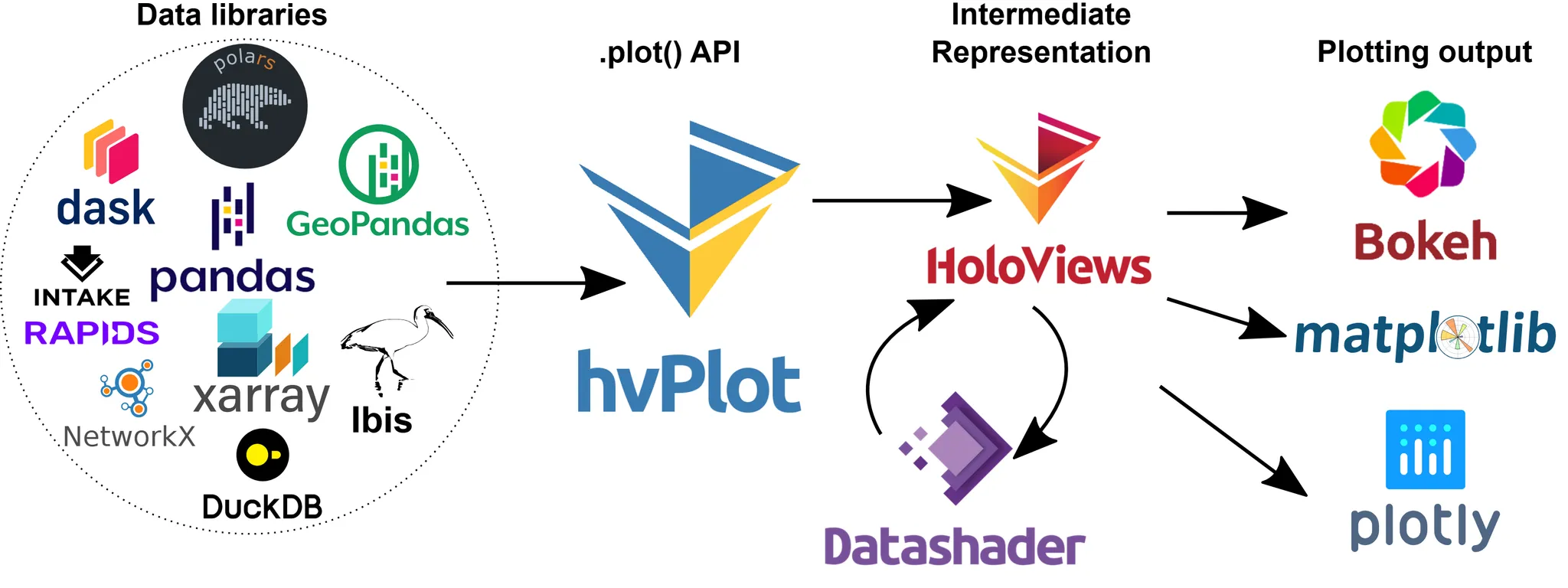
UXarray can use different backends. The default is bokeh which produces fancy interactive graphs. If we add backend='matplotlib' in the plot function, it would use matplotlib .

The default view is very small. So we can use height and width to adjust it. This is implemented not in bokeh but in hvPlot .

3. Add a background map (for Bokeh)

See also: Plotting

UXarray recommends the GeoViews package, which is a wrapper of our good old Cartopy.

import cartopy.crs as ccrs
import geoviews.feature as gf

(uxds['rainc'].isel(Time=TIME)
+uxds['rainnc'].isel(Time=TIME)
).plot(projection=ccrs.PlateCarree(),
       # backend='matplotlib',
       aspect='equal',
       height = 900,
       width = 1600,
      )*gf.coastline(scale='50m',projection=ccrs.PlateCarree())

geoviews.feature can be used just the same as cartopy.feature. So here I set the scale to be 50m (better resolution). Don’t forget to set the projection as well!

Extra: plotting the mesh

Reference: Link

You can easily plot the mesh like this:

grid_path = "../../test/meshfiles/ugrid/quad-hexagon/grid.nc"

data_paths = [
    "../../test/meshfiles/ugrid/quad-hexagon/random-node-data.nc",
    "../../test/meshfiles/ugrid/quad-hexagon/random-edge-data.nc",
    "../../test/meshfiles/ugrid/quad-hexagon/random-face-data.nc",
]

uxds = ux.open_mfdataset(grid_path, data_paths)
uxgrid = uxds.uxgrid

uxgrid.plot.edges(color="black", title="Grid Edge Plot")

It is quite GPU intensive.